Introduction

Dawson function, or Dawson integral, F(x) is an entire function [1,2,3] best defined as

(1)   

and shown in this Figure:

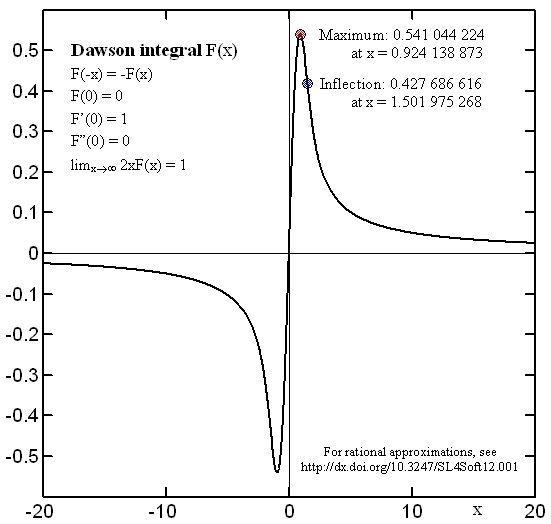
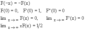
It is an odd function, characterized by the following behavior [1,2,3] for very small and very large values of the argument (needles to say, these features should be respected exactly by any numeric approximation):

(2)   

Closely related [4,5,6] is the imaginary error function erfi(x),

(3)   

whose numeric values are in fact best computed from the Dawson function:

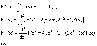
The derivatives of the Dawson function [7] are also best computed directly from its own values:

(4)   

The integral of F(x) is more complicated (for large x it grows as O[ln(x)]) and, if needed, should be evaluated using a different approximation.

The general shape of the Dawson function resembles x/(1+x²), i.e. the "imaginary" part of a Lorentzian peak profile, except that at large values of x it tends to zero as 1/2x rather than 1/x.

This fact is a good indication that an efficient and precise rational function approximation should be possible.

Computation of exact values

To provide a reference for the fitting of approximation parameters, as well for the respective maximum error estimates, it is necessary to be able to compute the values of the approximated function to a precision much better than that of the approximation.

For sufficiently small values of the argument, F(x) can be evaluated using the well known series expansion [1], while for large values one can resort to the asymptotic series [3, formula 7.1.23], provided appropriate care is taken to avoid propagation of rounding errors. Another approach is to use continued fraction expansions of which the most suitable one is that of Eq.(14) in reference [1], due to McCabe [8]:

(5)   

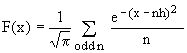
Still another method to compute F(x) for any x is due to G.B.Rybicki [9], based on the following formula

(6)   

which holds for arbitrary positive h and is exponentially convergent when h is small. There are of course several alternative methods [see references in 10], but they were not explored here because the scope of this study is the development of fast-executing approximations rather than a comparative evaluation of ultra-high precision evaluations. Sufficiently precise values are needed only as a reference for the optimization of numeric coefficients.

The Rybicki formula had been cast into an algorithm and recommended by Recipes in C [10, chapter 6.10]. For the purposses of this work, the Recipes algorithm has been tested for maximum error and consequently modified to improve its error. The modified code, evaluated in double precision has maximum relative error below 1e-15 (compared to 5e-8 of the original version). The modification will be described in a subsequent article.

In the end, the 'exact' value algorithm employed for the present work was an implementation [see ref.3, section 3.10.1] of the continued fraction of Eq.(5). It can be made arbitrarily precise and it is reasonably efficient (requires at most 30 steps to reach 15 digits precision), performs excellently for both very small and very large argument values (tested from 0 to 1000), and it is quite robust with respect to rounding errors. It's real-valued version (double) is made available here in the "C" package.

Proposed approximations

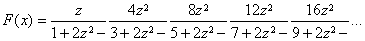
We approximate F(x) by rational functions of the type

(7)   

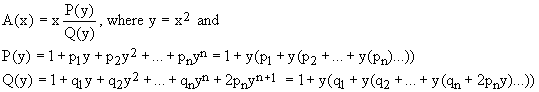
which guarantee the correct behavior small and large values of x.

The second forms for the polynomials P(x) and Q(x) illustrate the efficient Horner's scheme of evaluation. In total, an evaluation of n-th order approximation formula requires 2n+3 multiplications, 2n+1 additions, and one division.

The value of n is called order of the approximation. The coefficients of the polynomials P(y) and Q(y) are numerically adjusted so as to minimize the maximum absolute or relative error over the interval [0,20], covered by a regular grid of 1000 test points.

Details of the employed fitting algorithm will be reported elsewhere.

Results

The following optimal coefficients and maximum errors were obtained for various approximation orders:

Order n = 1

Optimized for best absolute error:
   p₁ = 0.3661869354
   q₁ = 0.8212009121
   maximum absolute error: 0.014 at x = 1.32;   (max.rel.err 6.79% at x = 2.90)
Optimized for best relative error:
   p₁ = 0.4582332073
   q₁ = 0.8041350741
   maximum relative error: 4.6% at x = 1.44;   (max.abs.err 2.2e-2 at x = 0.62)

Order n = 2

Optimized for best absolute error:
   p₁ = 0.1264634385   p₂ = 0.0734733435
   q₁ = 0.8234288542   q₂ = 0.2548465663
   maximum absolute error: 1.2e-3 at x = 2.36;   (max.rel.err 1.02% at x = 4.74)
Optimized for best relative error:
   p₁ = 0.1329766230   p₂ = 0.0996005943
   q₁ = 0.8544964660   q₂ = 0.2259838671
   maximum relative error: 0.52% at x = 5.15;   (max.abs.err 2.76e-3 at x = 1.06)

Order n = 3

Optimized for best absolute error:
   p₁ = 0.1154998994   p₂ = 0.0338088612   p₃ = 0.0106523108
   q₁ = 0.7790120439   q₂ = 0.3023475798   q₃ = 0.0533374765
   maximum absolute error: 1.19e-4 at x = 6.09;   (max.rel.err 1522 ppm at x = 6.97)
Optimized for best relative error:
   p₁ = 0.1349423927   p₂ = 0.0352304655   p₃ = 0.0138159073
   q₁ = 0.8001569104   q₂ = 0.3190611301   q₃ = 0.0540828748
   maximum relative error: 693 ppm at x = 3.70;   (max.abs.err 3.67e-4 at x = 0.78)

Order n = 4

Optimized for best absolute error:
   p₁ = 0.0989636483   p₂ = 0.0416374730   p₃ = 0.0047331350   p₄ = 0.00128928851
   q₁ = 0.7658933041   q₂ = 0.2834457360   q₃ = 0.0707918649   q₄ = 0.00827315960
   maximum absolute error: 1.37e-5 at x = 1.54;   (max.rel.err 165 ppm at x = 9.85)
Optimized for best relative error:
   p₁ = 0.1107817784   p₂ = 0.0437734184   p₃ = 0.0049750952   p₄ = 0.0015481656
   q₁ = 0.7783701713   q₂ = 0.2924513912   q₃ = 0.0756152146   q₄ = 0.0084730365
   maximum relative error: 90.0 ppm at x = 3.42;   (max.abs.err 4.87e-5 at x = 0.92)

Order n = 5

Optimized for best absolute error:
   p₁ = 0.1048210880   p₂ = 0.0423601431   p₃ = 0.0072584274   p₄ = 0.0005045886   p₅ = 0.0001777233
   q₁ = 0.7713501425   q₂ = 0.2908548286   q₃ = 0.0693596200   q₄ = 0.0139927487   p₅ = 0.0008303974
   maximum absolute error: 2.14e-6 at x = 1.42;   (max.rel.err 11.2 ppm at x = 3.38)
Optimized for best relative error:
   p₁ = 0.1049934947   p₂ = 0.0424060604   p₃ = 0.0072644182   p₄ = 0.0005064034   p₅ = 0.0001789971
   q₁ = 0.7715471019   q₂ = 0.2909738639   q₃ = 0.0694555761   q₄ = 0.0140005442   p₅ = 0.0008327945
   maximum relative error: 10.1 ppm at x = 1.78;   (max.abs.err 3.78e-6 at x = 0.72)

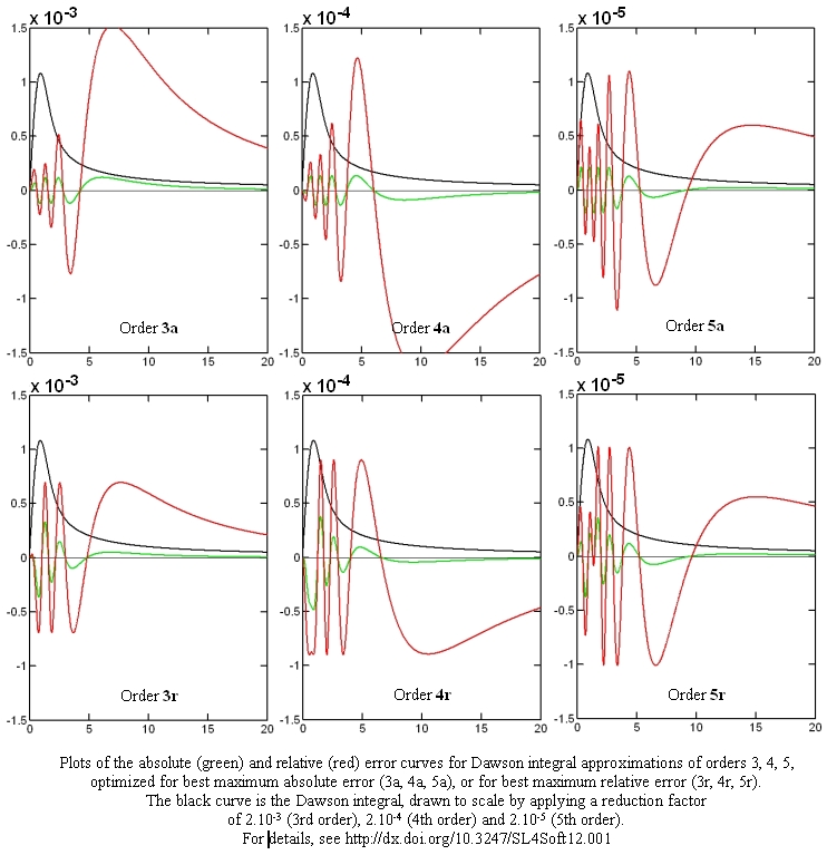
Error plots

The following Figures show the absolute (red) and relative (green) error curves for the rational approximations of 3rd, 4th and 5th order:

Conclusions

The approximations of orders 1 and 2 are probably too crude to be used in any practical application; they are listed here only for the sake of completness. However, the approximations of orders 3, 4, and 5 are certainly quite usable, offering also the possibility to struck a compromise between precision and speed (number of operations). The precision increases by a factor of almost ten from one approximation order to the next (at the cost of two more multiplications and two additions). It was not possible to go beyond order 5, though, because of numeric convergence problems encountered during the fitting of the coefficients (work in progress). The error plots 4th and 5th order approximations show small irregularities at low values of the argument, indicating that they, too, might have fitting convergence problems and, once those are overcome, a slightly better approximation coefficients might be found.

It is comforting that the optimal coefficients for either absolute or relative maximum error are similar and that they vary in a regular way from one approximation order to the next one. This indicates that they are "significant" and not conditioned by an "unnatural" starting assumption or by limited precision. Likewise comforting is the fact that the maximum errors occur for moderate x values in the central part of the fitted interval rather than at its extremes, thus indicating that they are indeed the worst deviations over the whole range of real-valued arguments.

The behaviour of the approximation formulas for complex arguments might be interesting but it was not yet investigated.

Comparing the present approximations to others, we have on one hand brute-force ultra-precise rational Chebyshev approximations [11] applicable piecewise to limited segments of the full argument range which have maximum relative errors of the order of 2e-20 or better. This is very nice but neither simple, nor elegant, nor particularly performant.

On the other hand, there exist very simple and fast approximations [12], but they are of overly limited precision, the best one having maximum relative error of 1.8e-3, worse than the order 3 approximations discussed here.

The approximations presented here are of extreme simplicity, both conceptual and practical. They cover the whole range of real numbers as arguments and utilize only the four basic arithmetic operations. The formulae are easy to implement on embedded microprocessors and can be even formulated as C macros. Finally, the approximations come in several versions with precisions ranging from very crude to more than satisfactory for all imaginable practical purposes (10 ppm). The availability of the choice of the maximum allowed error may be in fact one of the principle strengths of this study.

Code annex

The C and Matlab codes for the used exact-value functions, and for the final approximations of orders 1 to 5 are provided below for a free download. The implemented approximations are those optimizing the relative errors. The EbDawson_C package includes a small self-standing Windows-compatible console utility to calculate the values of the Dawson function with 17 digits precision as well as all five approximations for any real argument value.

• EbDawson_C.zip  ... The C/C++ functions, and the console utility.
• EbDawson_M.zip ... The Matlab functions.