|
Introduction
Temporary note: This is the first article in the Know Thy Spins series and, in a sense, it starts in the middle of the topic. The notation iso(AB) indicates a coupled AB spin system composed of two spin 1/2 nuclides under the isotropic rapid-tumbling conditions (liquid-phase high-resolution spectroscopy). Possible alternatives would be axo(AB) for axially oriented systems, spd(AB) for solid powder, and scr(AB) for a single crystal. Also, I take the iso(AB) peak frequencies and intensities for granted, relying on the many textbooks in which they are derived. With time, these gaps will be closed, making the Know Thy Spins series a self-coherent, closed exposition of the coupled spin-systems topic. As the work proceeds, the articles will get updated, especially for what regards hypertext links and comments like this one.
The geometric rules applicable to the iso(AB) quartet of spectral peaks are possibly stated here publicly for the first time. They are no big science, rather, we might call them recreational NMR, in the same sense in which one uses the term in Math. I was using some of these tricks back in the sixties and never thought about publishing them, considering them too obvious for a scientific article. Recently, discussing casually with a young friend, I realized that he was surprised by the existence of such rules, and even amazed by the fact that something useful could be done in NMR using just a compass and a ruler. Hence this article which, in addition, includes also a few comments of a more general nature on those features of the iso(AB) multiplet which have a more universal validity.
Transition frequencies and intensities in an iso(AB) spin system
The spectrum of an iso(AB) spin system is well known and described in almost every basic-level NMR textbook. It consists of four transitions which can be usually experimentally resolved as four distinct spectral peaks. The parameters of the spin system include two chemical shifts s(A) and s(B), and the scalar coupling constant J(AB). Without any lack of generality, we can assume s(A) ≤ s(B) and reference the spectrum so that [s(A)+s(B)]/2 = 0. This leaves just two parameters, the coupling constant J and the difference of the chemical shifts Δ = s(B)-s(A), which determine the positions and intensities of the spectral peaks.
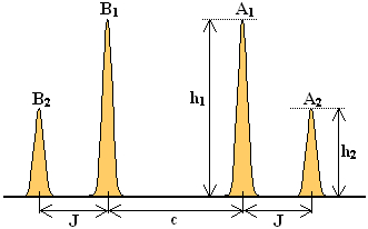
Expressing both parameters in frequency units [Hz], the four peak positions and intensities are:
| Transition T | Frequency f(T) | Intensity h(T) |
| A2 | - (c/2)-J | 1- k |
| A1 | - c/2 | 1+k |
| B1 | +c/2 | 1+k |
| B2 | +(c/2)+J | 1- k |
 |
|
 |
The value of k is always comprised between 0 (two singlets with no coupling) and 1 (an equivalent A2 group).
It can be used to roughly classify the strength of the AB system's coupling as:
# very weak with k < .0005 (Δ greater than about 200 J): peak intensities do not differ by more than 1%,
# weak with .0005 < k < .05 (Δ between 20 J and 200J): peak intensity differences are below 10%,
# moderate with k intermediate between weak and strong (see the next case).
# strong with k > 0.818 (Δ smaller than about 0.7 J): outer peaks are smaller than 10% of the inner peaks,
General characteristics of the iso(AB) quartet
A simple inspection of the table of transition frequencies and intensities reveals the following facts:
- The quartet is symmetric with respect to its center and ...
- ... it is invariant with respect to the change of sign of J.
- When J changes sign, so does k. The result is a permutation between pairs of peaks (A1 with A2, and B1 with B2) which involves both the frequencies and intensities and thus leaves the quartet spectrum invariant.
Consequently, it is impossible to determine the sign of J from the AB quartet spectrum. If one finds the parameters (D,J) which fit the spectrum, an identically good fit is obtained also for the parameters (D,-J). This is the simplest case of multiple solutions to the inverse problem of determining spin system parameters from its experimental spectrum.
Knowing this, we will henceforth assume J ≥ 0 but keep in mind that its true value might be negative.
- The distance (splitting) between each outer peak and its corresponding inner peak is exactly J.
- This apparently fortuitous fact indicates two more general facts:
(a) There is an A-group splitting with the same value as a B-group splitting. This constitutes the simplest example of a universally valid shared splitting theorem which will be discussed elsewhere in this series.
(b) Regardless of how strong is the coupling, the splitting is always the same as in a simple-minded first order analysis. Again, this illustrates a general tendency: when it comes to the values of splittings, Nature tends towards first order. However, be aware: nothing of the kind applies to absolute positions of the peaks and, especially, to peak intensities. And in systems more complex than AB, the statement is just an approximation.
- The outer peaks are never more intense than the inner peaks.
- This fact is better known as the roof effect. In the AB quartet it is very clear and simple, but it persists also in more complex multiplets, where it assumes a more statistical character.
- When Δ tends to 0, the two inner peaks tend to coalesce and the outer ones tend to vanish.
- In the limit case of Δ = 0, the AB system becomes a group A2 of two equivalent nuclides (notice that the transition from AB to A2 is continuous). Once this happens, the two outer peaks have zero intensity and can't be observed so that there is no way to determine the value of J (the spectrum becomes insensitive to it). This is the reason behind the ubiquitous but totally wrong statement that "equivalent nuclides do not couple" which reflects a mental confusion between the two predicates "data are insensitive to J" and "J is zero".
In this context, it is interesting to consider what happens when Δ is small (Δ << J) but not zero. In such cases we have a central doublet with a small splitting of about Δ*(Δ/2J) and weak outer peaks with relative intensity of about (Δ/2J)2. On high field instruments (where we typically have a high S/N but a bad digital resolution) there is a limit below which the outer peaks are still visible but the central doublet is no longer resolved, so that the multiplet looks like a triplet with pathological intensities (you might misinterpret it as a fortuitous superposition of a singlet with a weak triplet). On low-field instruments (modest S/N but good spectral digitization) the opposite can happen: the outer peaks are lost in noise and what remains visible is a misleading, resolved central doublet whose splitting does not reflect any valid J (it actually decreases with increasing J). Notice that insistent accumulation will eventually lead to a resolution of the low-field impasse (since the weak peaks will start showing) while the high-field misinterpretation will persist forever!
The case we are discussing is also important in spectral fitting. In strongly coupled AB systems, the spectrum becomes quite insensitive to variations in J - and even more so to correlated Δ and J variations in which Δ*(Δ/2J) remains constant. This implies large experimental errors in the fitted values of both J and Δ. In addition, it also indicates that when some strong couplings are present in a spin system, the errors in the estimated spin system parameters may vary dramatically from one parameter to another and, as a further complication, they may be strongly correlated.
Rule I: A constraint on peak intensities and its geometric representation
Using the explicit formulas for peak frequencies and intensities and applying elementary arithmetics, one easily finds out that:
The ratio of the intensity of the inner peaks to that of the outer peaks equals the ratio of the separation between the outer peaks to that between the inner peaks, i.e., h1/h2 = (2J+c)/c = [f(B2)-f(A2)]/[f(B1)-f(A1)].
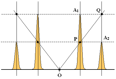
Geometrically, this implies a constraint between peak positions and intensities or, depending upon one's point of view, a geometric test of whether a given symmetric quartet is compatible with an AB system (see the Figure on the right):
Find the center O of the quartet at the baseline level. Now mark the point P which has the same frequency as the A1 peak but the height of the A2 peak. Mark further the point Q which has the same frequency as the A2 peak but the height of the A1 peak. Then the points OPQ must lay on a straight line segment. Given the symmetry of the quartet, an analogous constraint applies also to the B-side of the quartet pattern.
Apart from the quartet's symmetry, this is the only constraint which there is. If you mark any four symmetrically disposed frequencies as the positions of the peaks of a hypothetical AB quartet, then Rule I fixes the relative intensities of the peaks. Beyond that, however, it is guaranteed that there exists a J and a Δ fully compatible with the resulting pattern (we will see shortly how to recover geometrically the value of Δ).
Practical uses of Rule I
First, it provides a simple method to draw correct sketches of AB quartets for lectures and other educational material :-)
Second, you can use it to test whether any four peaks which look like an AB quartet actually might be one. The two conditions to keep in mind are (i) the common numeric value of the separation between each outer peak and the corresponding inner peak (the J) and (ii) the present rule for peak intensities. Naturally, one must take into account possible errors due to noise and baseline artifacts, but that is rather obvious. Rule I is particularly good when it comes to excluding false positives: if an AB-like quartet violates it, it is not an AB quartet!
Third, given two peaks which possibly might be one half of a quartet (say, the A-peaks) the rule can be used to find the expected location of the B-peaks. Just mark the points P, Q in the A-group, draw the line passing through them and find where it crosses zero (or the true baseline). This should be the center O and you just need to reflect the two A-peaks about O to obtain the expected locations and intensities of the B-peaks. It is great in those cases when the B-peaks fall inside a crowded region. Again, of course, you must take a reasonable care of possible errors due to noise and other artifacts (this becomes particularly critical when the coupling is weak and the B-peaks are distant).
In the last case, the a-priori knowledge (or assumption) that the two peaks A1, A2 belong to the A-multiplet of a coupled AB system allows us to reconstruct also the "remote" B-multiplet. This interesting possibility, present also in more complex spin systems, is characteristic of moderately to strongly coupled systems. In weakly-coupled systems the distance to the remote multiplet becomes ill defined (but one can at least place a lower limit on it).
Rule II: Geometric determination of the chemical shift Δ from peak positions
The chemical shift between the two nuclides A and B is buried in a formula involving a square root. Nevertheless, it is easy to recover it using just a compass and a ruler. Using the following Figure, let us start with the recipe and then prove that the construction is correct.
Construction:
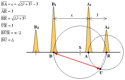
All we need are the three points A, B and R which mark respectively the positions of the central peaks A1 and B1 and of the rightmost peak A2 (equivalently, one could also use the leftmost peak). Use the compass and the ruler to find the center S of the segment BR (hopefully, everybody knows how to do it). Now draw two circles: one with its center in S and passing through B and R, the other with its center in R and passing through A. Denoting one of the intersections of the two circles as U, the desired chemical shift difference Δ is the length of the segment BU.
Proof:
The proof is contained in the six equations shown in the Figure. The first two follow directly from the formulas listed in the Table of peak frequencies and intensities. The third one (the distance BR) is the sum of the first two. The fourth one holds since, by construction UR = AR. The fifth says that the angle BUR is right which is true because it is the inscribed angle above the diameter of the circle with center S (see Thales' theorem). The right-angled triangle BUR therefore has a hypothenuse BR of the length given by the third equation and one side, RU whose length equals J. It then follows from the Pythagoras' theorem that the length of its remaining side BU must be Δ. QED.
There are two facts that should be noticed:
(a) The construction recovers the value of Δ but not the "decoupled" chemical shift positions of the individual nuclides A and B. If need be, those can be determined by bisecting the segment BU to find s = Δ/2 and then marking the two points at distance s upfield and downfield of the quartet's center.
(b) The diameter BR of the circle with center in S coincides with the value for the difference of the chemical shifts determined by first-order analysis. The effect of strong-coupling on this parameter is therefore embodied by the difference between the length of the red line (also a chord of the same circle) and the said diameter.
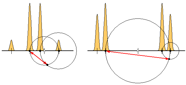
It is fun to play with the construction, especially with the limit cases of very strong (below left) and weak (below right) coupling. The first case reveals the coalescence behavior (quite large Δ even with a small separation c between the central peaks) while in the latter case the chemical shift tends towards BR (as expected from first-order analysis).
Evidently, one can combine the two Rules to reconstruct the chemical shift difference Δ from just the two A-peaks. It is sufficient to use Rule I to find the center of the quartet and the position of the B1 peak and then proceed according to Rule II. In weakly coupled AB systems and the presence of noise, the construction may become too imprecise, but otherwise it is not bad.
Geometric construction of the [Δ,J] quartet
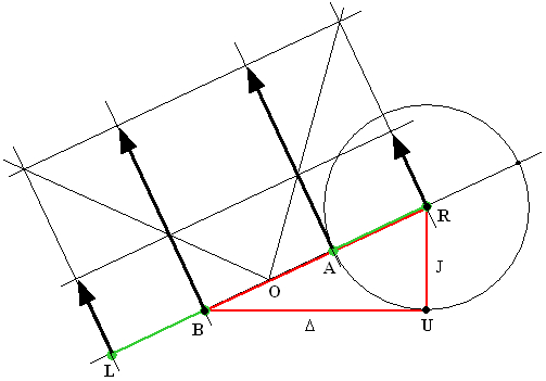
As a final case, suppose that we are given the values of Δ and J and asked to draw the corresponding AB quartet. The construction, shown on the right is in a certain case a reverse of the case discussed in the last Section. Construct first a rectangular triangle BUR with the sides BU = Δ and RU = J. The hypothenuse and its straight line extension will be our baseline. Use the compass to mark the point A on the hypothenuse such that RA = RU. Now the points B,A,R correspond to the positions of the peaks B1, A1 and A2, respectively, and the point L on the extended hypothenuse such that BL = RA corresponds to the position of the peak B2. Draw four lines perpendicular to the hypothenuse and passing respectively through the four points L, B, A, R. Now bisect the segment BA to find the center O of the quartet and apply Rule I to define the relative peak heights.
A simple real-world example using really old data
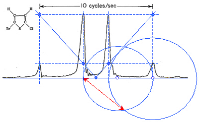
The spectrum on the right comes right from the 1959 book of Pople, Schneider and Bernstein, so I guess that it was measured around 1956. The spectrometer frequency was 30.7 MHz and the instrument operated in CW (continuous wave). All the black parts of the Figure are original - I have simply scanned them from the book. The blue lines were overlayed by myself and represent the application of Rule I which confirms that the quartet might indeed belong to a coupled AB system. The blue circles constitute the application of Rule II and their intersection defines the chemical shift difference equal to the length of the red double-arrowed line. Compared to the 10 Hz marker supplied with the original data, this turns out to be 4.7 Hz which is exactly the value reported in the book.
A somewhat more complex real-world example
The next Figure is a screenshot of a portion of a 250 MHz spectrum of the shown compound. The displayed region comprises the peaks of the coupled protons 5 (right half) and 6 (left half), both of which are weakly coupled to proton 2 through long-range couplings. We can virtually remove the long-range couplings by replacing each narrow doublet with a virtual peak such that its position matches the center of the doublet (thin vertical lines) and its height matches the average height of the doublet's local maxima (thin horizontal lines).
To test whether the result might correspond to an AB-type quartet, we first verify that the outer splittings are indeed the same (the two green double-arrow lines have the same length). Next we apply Rule I separately to each side and find that it holds (the two blue double-arrow lines of the same length are used just to indicate the center of the pattern). There is just a barely perceptible discrepancy at the right side, probably due to the fact that the long-range coupling slightly falsifies the heights (it would have been better to work with integrals). By and large, the agreement is excellent and the hypothesis that we have here a coupled AB system with further fine splittings on both nuclides can be accepted. Since the coupling in this quartet is quite moderate, the chemical shift estimated by Rule II (the red double-arrow line) differs only marginally from the value derived from first-order analysis (the diameter of the bigger circle).
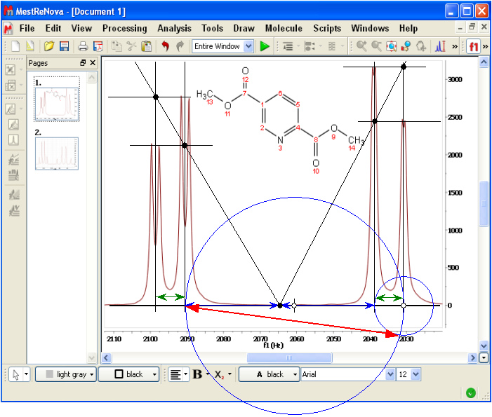
Note: This test was carried out directly on a screenshot of a commercial Application window. The thin vertical and horizontal lines, the black dots, the green, blue and red double-arrow lines and the circles are not part of the screenshot; they were added after the screenshot was imported into a Word document. There were better ways to do it (for example, using the Application's incorporated drawing facility) but this primitive approach somehow better conveys the fact that the two rules can be easily applied to any hardcopy scrap of a spectrum.
A word of warning
We have so far identified peak heights with transition intensities. This may not be completely correct since the linewidths of the inner and the outer peaks in an AB quartet need not be the same. Especially in strongly coupled AB systems the natural linewidths of the weak outer peaks are considerably smaller than those of the inner peaks so that they may appear taller than expected (this is due to the properties of the relaxation matrix of the coupled system). Whether this natural linewidths difference will be detectable depends upon magnetic field inhomogeneity (inhomogeneity affects all peaks and thus tends to mask any differences).
In order to avoid such doubts, one should use peak integrals rather than peak heights.
|