|
Approximations which require the evaluation of a single square root (class S)
Let us re-consider approximations which are exact for both the circle (y = 1) and the degenerate flat ellipse (y = 0). Like in the case of purely algebraic approximations [1, A1 to A7], we will require that our formulas (i) be invariant under the permutation of the two axes a,b and (ii) exhibit proper dimensional (scaling) behavior. This time, however, we will allow not only the operations of sum (+), subtraction (-), product (*) and division (/), but also that of a square root, provided that the formula calls for just a single square-root evaluation.
Following the line of reasoning discussed in [1], all such approximations can be reduced to the general, rationalized form
(1) 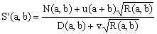 , ,
where D(a,b), N(a,b) and R(a,b) are polynomials in the semi-axes a,b which are fully symmetric under their exchange (so is, evidently, the first-order factor (a+b)). When the degree of D(a,b) is n, then the degrees of N(a,b) and R(a,b) must be (n+1) and 2n, respectively. As in [1], we will use the value of n, combined with the letter S, to classify and label these approximations.
As usual, each formula for S'(a,b) gives rise to an approximation E'(x) for the complete elliptic integral of the second kind by (i) dividing S'(a,b) by 4a and (ii) setting y = a/b, with y being also identical to √(1-x) [reference 2, Eq.(6)].
Each of the approximations S0, S1, etc. leaves free a certain number of coefficients whose values are subject to two boundary conditions S'(a,b), namely S'(a,0) = 4a and S'(a,a) = 2π. When the total number of coefficients is c > 2, this leaves (c-2) adjustable coefficients. Here we use brute force and fit such coefficients so as to minimize the maximum error over the whole interval [0,1] of y-values of interest and report the optimize error's upper bound and the corresponding coefficients.
Only the approximations S0, S1 and S2 have been investigated since optimization of the higher ones is extremely difficult (slow and uncertain convergence). It turns out that all three approximations are new, but S1 is very closely related to an earlier one, proposed by D.Cantrell (Cantrell 2004). S1 can be in fact reduced by pre-setting one of its coefficients with just a minor effect on its maximum error; the resulting approximation is then practically identical to Cantrell's.
Figure 1 shows the error curves of all the approximations named above, plus some which do not fall into this family but also use just one square root. When comparing the various approximations, we will consider the square root operation equivalent to about 10 arithmetic ones (an initial estimate, plus 4 Newton's formula iterations). When comparing them to the purely algebraic ones, it means that Sn executes about as fast (or faster) as A(n+3).
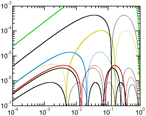
Figure 1. Relative error curves of Class S approximations
The curves ε(y) are plotted against y.
The bold sections of each curve indicate that the approximate value is greater than the exact one, while a thin trace indicates that it is smaller. The curves are distinguished by color and by their maximum error value. The following 'old' approximations were listed in [2] in other categories, but they belong also to this one: Takakazu Seki Kowa (E3, green, 13500 ppm), Rivera II (C3, yellow, 103 ppm), Cantrell-Ramanujan (C6, blue, 14.5 ppm). The approximations discussed here are: S0 (black, 430 ppm), S1 (black, 3.241 ppm) and S2 (black, 0.858 ppm). The red curve (4.134 ppm) corresponds to the reduced S1 approximation, identical to Cantrell 2004 (see below).
*** S0 approximation; maximum error 429.9 ppm
(S0) 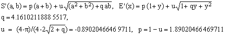 . .
This new approximation satisfies all our requirements, even though it does not exactly conform to Eq.(1) because, since its denominator is simply 1 (order 0), it does not contain the (a+b) multiplier of the square root term. It has the total of three parameters, of which only one is adjustable.
The maximum error may not look very impressive but consider that, in order to get comparable precision, one must resort to the purely algebraic formulae A2 (557.3 ppm) or even A3 (15.3 ppm) which, in terms of computational efficiency, appear similar or worse.
*** S1 approximation; maximum error 3.241 ppm
(S1)  . .
Now, this is an impressive improvement! In a sense, the square root term in the formula can be viewed as a correction of the first-order algebraic approximation A1 which, however, has a maximum error of 6313 ppm. To reach a comparable precision with purely algebraic expressions, one needs to use at least the numerically less efficient fifth order (A5, 3.65 ppm).
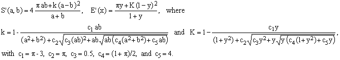
*** S2 approximation; maximum error 0.858 ppm = 858 ppb
(S2) 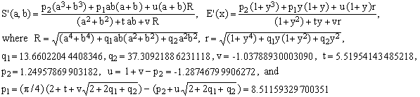 . .
This new approximation is again a progress. After A6 it is the second approximation to break the 1 ppm maximum error barrier and it is numerically more efficient. However, comparing it with the preceding one (S1) or with A2 (557.3 ppm) which it corrects, the drop in maximum error is smaller than in the case of S1.
Cantrell 2004 revisited: geometric insight against brute force
It is evident that there is something in these approximations (particularly in S1) that confers them an exceptional performance.
A closer look at the Cantrell 2004 formula,
 , ,
reveals that it belongs to class S and is of first order. To make S1 and Cantrell 2004 fully equivalent, it is sufficient to put p2 in (S1) equak to 1 instead of the optimal value 0.99983... I therefore believe that what we see here is an underlying approximate geometric principle which David Cantrell guessed through a sound combination of reasoning and intuition.
Even when p2 = 1 in (S1), one can still adjust the remaining coefficients q and v, obtaining the following reduced S1 formula:
(S1r) 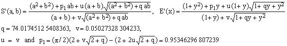 , ,
which coincides with Cantrell's for w = 74.00393846 and p = 0.410117999. The maximum error of 4.134 ppm is only slightly worse than that of S1 (3.241 ppm) and practically identical with that reported by Cantrell (4.159 ppm). The marginal difference between the two values is due exclusively to the quirks of the idle parameters optimization process (Cantrell's values were w = 74 and p = 0.410117).
Errata Corrige: I wish to put straight an error of mine. In the 2005 Review [2] I have made an error in copying the value of the parameter p (0.2410117 instead of the correct 0.410117). Consequently, my Matlab software gave me a very bad maximum error and made me to mis-classify the formula as E2.
Ahmadi 2006: another breakthrough approximation based on insight
In an e-mail to David Cantrell dated January 30, 2007, Mahmood Shalil Ahmadi, a chemical engineer working at a power station in Bandar Abbas, Iran, proposed a very precise new approximation. David councelled Mahmood on a couple of points and forwarded the e-mail to me. I have exchanged a couple more e-mails with Mahmood, trying to understand how he arrived at the formula. Frankly, it is still not quite clear to me, but that must be due to mine being obtuse, since the formula works beautifully. What transpires clearly from Mahmood's notes is the fact that he combined geometric insight with symmetry & scaling requirements, plus quite a lot of guesswork. But let us see the result:
*** Ahmadi 2006; maximum error 2.3713 ppm
Though its author probably did not notice, the formula can be interpreted also as a corrected Cantrell's Particularly Fruitful approximation [ref.1, E5], the correction consisting in allowing the factor k to deviate from 1. The art, of course, lies in guessing the best functional form of the deviation with its two nested square roots.
A surprising feature of the Ahmadi formula is the lack of any adjustable parameters, with all numeric coefficients having simple, fixed values (by itself, this is a tribute to Ahmadi's insight). Since we are talking about approximation, however, there is no reason why the coefficients should not be fine-tuned to improve its precision. I have therefore tried and numerically adjusted the parameters so as to minimize the maximum error. The result is the best known approximation up to this date:
*** Optimized Ahmadi; maximum error 0.1516 ppm = 151.6 ppb
c1 = 0.14220038049945, c2 = 3.30596250119242, c3 = 0.00135657637724, c4 = 2.00637978782056, c5 = 5.3933761426286;
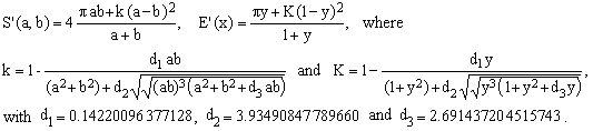
Noticing that c3 is very close to 0, I have also tried to eliminate it altogether. This allows a functional simplification and leads to a reduced form with just three adjustable parameters and, after a new fitting, turns out to have practically the same maximum error as the previous case (actually, for y > 0.25, it is better), while being computationally more efficient:
*** Reduced Ahmadi; maximum error 152.0 ppb
The error functions of Ahmadi 2006 and its optimized and reduced forms are plotted in Figure 2 which,
for comparison, shows also all presently known approximations with maximum relative error smaller than 10 ppm.
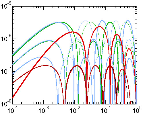
Figure 2. Error curves of approximations with maximum relative error < 10 ppm
The light-blue curves are the purely algebraic approximations A5, A6 and A7 of orders 5, 6 and 7 (ordered by decreasing maximum error). Of these, A5 is equivalent to Cantrell 2006 [see 2b]. The two light-green curves correspond to the S1 and S2 approximations introduced in this article, of which S1 is practically equivalent to Cantrell 2004. The red trace shows the error curve of the original Ahmadi 2006 approximation, while the darker red-brown trace belongs to optimized Ahmadi which is currently the best known approximation. It practically overlaps with the reduced Ahmadi approximation except at large y-values where the reduced form is better (thin black trace).
Conclusions
Considering the rapid progress of ellipse perimeter approximations in the last two years (Cantrell 2006, the purely algebraic A-class forms, the S-class with one square root, and the Ahmadi group), we have left behind our shoulders the 1 ppm barrier and are pointing towards 100 ppb or even 10 ppb.
At this point, one really should review the question of numeric efficiency of all the approximations and weed out those which, in any given maximum-error class, are overshadowed by more efficient ones. This task is not quite as simple as it sounds and will be done in a separate article. However, there is now little doubt that the reduced Ahmadi and some of the S-class approximations (including Cantrell 2004) will hold prominent places in such a hierarchy, while the importance of the A-class seems to be diminishing.
|