Introduction

Let (X,Y) be the Cartesian coordinates of a plane. Then the equation

(1)   

defines an ellipse with semi-axes a and b, assumed to be non-negative real numbers.
For the purposes of this review, we will also assume that a > b.

From the geometric point of view, any planar curve obtained from Eq.(1) by means of a rotation and a translation is also an ellipse. Such operations correspond to replacing the coordinates (X,Y) with

(2)   

where α is the rotation angle and (X₀,Y₀) the translation vector.

Given the invariance of distances under rotations and translations, all such ellipses are equivalent in the sense that they have the same semi-axes, perimeters and areas. Vice versa, any ellipse belonging to this family can be brought to the normal form of Eq.(1) by a suitable translation and rotation. There are ways to define all such ellipses in free form (i.e., with no reference to any particular coordinate system) and study their coordinate-free geometric properties. This, however, is not the purpose of this review and an interested reader is invited to consult alternative sources such as the 'ellipse' entry in Wikipedia.

Using elementary integration methods, the perimeter S(a,b) of the ellipse defined by Eq.(1) turns out to be

(3)   

is the ellipse eccentricity and

(4)   

is the complete elliptic integral of the second kind, a well known mathematical entity [1,2,3] which can be computed with relative ease using, for example, numeric integration or brute-force rational approximations [1] or the Carlson's algorithms described in [3].

The problem with Eq.(3) is that E(x) is a transcendental function and its evaluation through infinite series or fractions is computationally inefficient, especially when implemented on simple microprocessors using floating point emulation software or hard-wired in FPGA's (Field-Programmable Gate Arrays). For this reason, various authors have proposed a number of approximations to S(a,b) using simple algebraic expressions or, at most, formulae containing only commonly used functions such as square root, generic powers, arctangent, etc.

General properties of the approximations

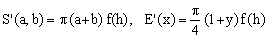
It turns out that in all known approximations the dimensionless entity S(a,b)/a can be expressed as a function of the ratio y = a/b. It is therefore convenient to rewrite Eq.(3) as

(5)   

This fact has several consequences. First, each approximation S'(a,b) for S(a,b) induces an approximation E'(x) for E(x) according to the formula

(6)   

Second, given the proportionality between E and S, the relative errors of the two approximations at the indicated argument values are the same. This means that plotting the relative error of E'(x) against y over its whole range [0,1], the maximum of the curve gives the maximum relative error of the approximation S'(a,b) for any pair of values a,b.

In the next Chapter we shall exploit such relative-error curves to compare and classify different approximations. In particular, we shall plot the quantity |ε(y)|, where

(7)   

The features of the error-curves which are most useful for classification purposes are their absolute maxima and their behavior close to y = 0 which is the extreme corresponding to degenerate ellipses with b = 0, e = 1 and S(a,0) = 4a. The approximations can be divided into two broad categories: those for which S'(a,0) = S(a,0) and those for which this is not true.

In this context it is interesting to note that all published approximations are exact when y = 1, which is the other extreme corresponding to a circle (b = a) for which the perimeter S(a,a) = 2πa is explicitly known. This may be due to the historic accent on trajectories of celestial bodies whose eccentricities tend to be relatively small.

In addition, approximations S'(a,b) using functions, no matter how simple and interesting they might appear, are much less useful in practice than those which employ only the four basic arithmetic operations of sum, subtraction, multiplication and division. This feature will represent another basis for our classification. In the case when only algebraic operations are employed, another parameter that should will be taken into account is the total number of arithmetic operations involved in evaluating the approximate expression.

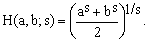
A number of approximations uses the parameter h defined as

(8)   

which ranges from 0 for circles (y=1, b=a) to 1 for the degenerate ellipses (y=0, b=0). This stems from the fact that there are three known infinite expansions for S(a,b), sometimes referred to as exact formulae and the one expressed in powers of h has the best convergence properties.

Before closing this Chapter, notice that the assumption b < a is quite artificial. Geometrically, the perimeter of an ellipse does not change when a and b are interchanged. One therefore strongly favors the symmetric approximations for which S'(a,b) = S'(b,a). Absolute majority of known approximations is indeed of this type.

K. Keplerian approximations

We will call Keplerian the approximations whose relative error curves attain absolute maximum at y = 0 (degenerate ellipses) and decay towards zero at y = 1 (circles). The name honors the astronomer Johannes Kepler (1571-1630) who in 1609 proposed the very first ellipse perimeter approximation which was of this type.

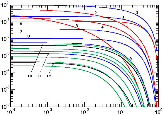
Figure 1. Error curves of Keplerian approximations 

Red color indicates that the approximate value is greater than the exact one (positive ε), while all other colors indicate that it is smaller (negative ε). The considered approximations are: 1) Kepler, 2) Sipos, 3) naive, 4) Peano, 5) Euler, 6) Almkvist, 7) quadratic, 8) Muir, 9) Lindner, 10) Ramanujan I (black), 11) Selmer II (blue), 12) Ramanujan II (black). Green curves correspond to the Padé approximations. From top down, these are: a) Selmer (Padé 1/1), b) Michon (Padé 1/2), c) Hudson-Lipka (Padé 2/1), d) Jacobsen-Waadeland (Padé 2/2), e) Padé 3/2, f) Padé 3/3.
 

The following paragraphs list, for each approximation, the formulas for S'(a,b) and E'(x). In the latter case, the right-hand-side is expressed in terms of y = b/a which relates to x as indicated in Eqs.[6,7]. The numbering of the paragraphs respects the numbering of approximations in Figure 1.

1) Kepler approximation

(K1)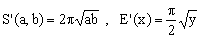   

This is the very first of many approximations which attempt to estimate the radius of the circle whose circumference equals the perimeter of the ellipse. Obviously, such an equivalent radius is a kind of mean value of the two semi-axes a,b.

Johannes Kepler used the geometric mean which in fact approximates the perimeters of the orbits of all celestial bodies he has observed with a precision far better than that of his measurements. The disadvantages of this approximation include a huge error (100%) in the degenerate case and, in addition, use of the square root function.

2) Sipos approximation

(K2)   

This 1792 approximation formula combines in an interesting way two means - arithmetic and Hölder - and achieves a precision for round ellipses (close to y=1) which is much better than Kepler's as well as that of the next two approximations. Unfortunately, its performance for flat elipses is less impressive.

3) Naive approximation

(K3)   

Interestingly, it turns out that simple arithmetic mean of the two semi-axes is a much better estimate for the equivalent circle radius than the geometric mean. Hence this approximation, referred to as naive by G.P.Michon and P.Bourke, even though it is more accurate and computationally more effective than Kepler's.

4) Peano approximation

(K4)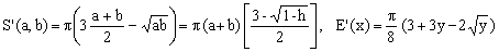   

One can interpret this Giuseppe Peano's 1889 approximation in two different ways, corresponding to the two expressions for S'(a,b). The first one is a combination of two means - arithmetic and geometric - based on the fact that two distinct types of mean can be combined to obtain a different one. It is interesting to see that a linear combination of two means can give rise to a markedly more precise approximation than each of them taken individually (compare K4 with K1 and K3).

The second form for S'(a,b) can be intended as the naive arithmetic-mean formula multiplied by a correction factor (the one in square brackets) according to the general scheme

(9)   

It appears that Peano originally followed the second line of reasoning (he used the parameter h), but both approaches are valid and we will encounter them again. Though Peano's formula requires square root, it appears justified since the increase in precision with respect to the naive approximation is quite remarkable for almost all values of y.

5) Euler approximation

(K5)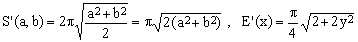   

The 1773 attempt, credited to Leonhard Euler (1707-1783), to replace the arithmetic mean with a quadratic mean is only moderately successful (Euler actually used it as a starting point for an exact expansion)). Compared with the naive approximation, it roughly halves the degenerate-case relative error, but the gain becomes negligible for y values greater than about 0.5. Considering the necessity to compute the square root, the rather modest increase in precision is hardly worth the trouble.

6) Almkvist approximation

(K6)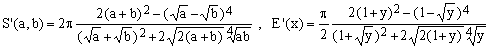   

For round ellipses, the 1978 approximation due to G.Almkvist is certainly much more precise than any of those listed above but the formula is particularly complex and therefore numerically inefficient.

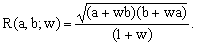
7) Quadratic approximation

(K7)   

is one which has been proposed and used by a number of authors. In a sense, it is a hybrid between Kepler's geometric-mean approximation (K1) and Euler's square-mean approximation (K5). One can, in fact, define a generalized quadratic mean Q(a,b;w) dependent on a 'mixing' parameter w

(10)   

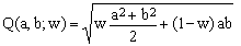
For any w, the mean Q(a,b,w) satisfies the mean-value condition Q(a,a,w) = a. Its special cases are the geometric mean for w = 0 and the square mean for w = 1. The best approximation for the ellipse perimeter is obtained with w = 3/4 (once again, the result is much better than the two special cases).

Like Peano's approximation, the quadratic one requires the evaluation of one square root. Since it is significantly better than Peano's for small values of y, it is certainly preferable (notice that for y > 0.5 the two approximations practically coincide).

8) Muir approximation

(K8)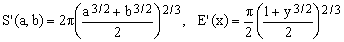   

This 1883 approximation by Thomas Muir (1844-1934) is based on the Hölder mean

(11)   

with the setting s = 3/2. We will hear more about Hölder means later on. For the moment it is sufficient to note that varying the single parameter s from minus infinity to plus infinity, one passes from min(a,b) to max(a,b), traversing on the way the harmonic mean (s = -1), the arithmetic mean (s = 1), and the square mean (s = 2). We have seen that the Euler's square mean approximation (K5, s=2) was slightly better that the naive arithmetic mean approximation (K3, s=1) but evidently one needs to move to an intermediate value of s to discover the vastly better optimum.

In terms of maximum relative error, Muir approximation certainly represents an improvement over what we have seen so far, but it requires the evaluation of two square roots and one cubic root or, alternatively, of three real powers (each requiring the evaluation of a logarithm and an exponent). From the computational point of view, Muir approximation is therefore rather inefficient.

9) Lindner approximation

(K9)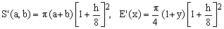   

This approximation, proposed by Lindner, possibly in 1904, is conceptually similar to Peano's in its second form in the sense that it uses the arithmetic mean and corrects it by means of a factor which is a function of h. In this case, the correction is equal to the first 3 terms of the Taylor expansion of the exact f(h).

Lindner's approximation is very successful, considering that it is much more precise than any of those considered above and that it involves only elementary algebraic operations. We shall not claim that it is the best one to use in practice only because the next one is even better.

10) Ramanujan I approximation

(K10)   

This 1914 approximation, due to the Indian mathematician Srinivasa Aiyangar Ramanujan (1887-1920), is often hailed as nearly miraculous. Actully, it is only marginally better than Selmer's and worse than the other Padé approximations to be discussed below. Moreover, compared to Selmer's formula, it uses the square root so that it is rather doubtful whether the slight improvement in precision can justify the considerable drop in efficiency.

What makes Ramanujan's first formula interesting to this Author is the fact that, like the first form of Peano's approximation, it can be interpreted as a combination of the arithmetic mean with another one, denoted as R(a,b;w) and defined by the equation

(12)   

In Ramanujan's formula we have w = 3 and the two means are combined linearly with relative weights +3 and -2, respectively.

11) Selmer II approximation

(K11)   

As far as maximum error is concerned, this E.S.Selmer approximation of 1975 is remarkably good. It certainly beats Rmanujan I by which it was clearly inspired. On the other hand, it is rather messy, less precise and numerically inefficient when compared, for example, with the Jacobsen-Waadeland Padé-type approximation to be discussed below.

12) Ramanujan II approximation

(K12)   

This is the second 1914 approximation due to Ramanujan. It is also of the generic type of Eq.(9), but it approximates f(h) by means of an innovative ad-hoc formula which, amazingly, matches all the Taylor expansion terms of f(h) up to order 9 (order 18 in terms of the eccentricity e)!

The precision of this expansion is very similar to that of Padé 3/2 (see below), with respect to which it is computationally slightly less efficient due to the presence of the square-root. Despite some of its clamorous aspects, therefore, Ramanujan II formula can hardly be considered as being particularly practical.

Padé approximations

This family of formulae (green curves in Fig.1) is based on approximating the correction term f(h) in Eq.(9) by rational functions following a method known as Padé approximants. We will not discuss the method in this Note; it is sufficient to know that it exists and that it consists in determining the coefficients of the rational function polynomials so as to match the largest possible number of terms in a known power-series expansion of f(h).

Padé approximations can be classified by fractions n/m, where n and m are the degrees of the polynomials in h appearing, respectively, in the nominator and denominator of the rational function. The simplest formula of this kind is the Selmer approximation of the type Padé 1/1.

Some of the lowest-degree Padé n/m approximations are associated with specific names. However, since the calculation of the coefficients of the rational function polynomials can be done automatically by computer algorithms, it is nowadays pointless to try and associate a name with all individual special cases.

Here is a list of some of the formulae based on Padé approximants (green curves in Figure 1):

Padé 1/1 (Selmer)

(Ka)   

Padé 1/2 (Michon)

(Kb)   

Padé 2/1 (Hudson-Lipka)

(Kc)   

This approximation was reported as a known one in a 1917 book by R.G.Hudson and J.Lipka.
Sometimes it is also referred as Bronshtein, 1964.

Padé 2/2 (Jacobsen-Waadeland)

(Kd)   

Padé 3/2

(Ke)   

Padé 3/3

(Kf)   

As expected, the precision of the approximations increases rapidly with increasing degrees of the rational function polynomials. Since all Padé approximations are pure algebraic expressions, they are also very practical and efficient.

O. Optimized equivalent-radius approximations

Some of the above approximations are based on equivalent-radius expressions which involve one or more adjustable parameters. In the preceding Chapter the values of such parameters were in general chosen so as to minimize relative error of the approximations in the vicinity of y = 1 (round ellipses with small eccentricity). However, one can adopt a different strategy and look for parameter settings which minimize the maximum error of the approximation across the whole range of possible y values. In this Chapter we will discuss a few such cases.

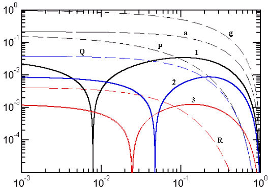
Figure 2. Error curves of several optimized equivalent-radius approximations 

Curve colors now link together families of approximations. The following cases are shown: Black-color group: g) K1 based on the geometric mean, a) K3 based on arithmetic mean, P) Peano K4 combining the two means and 1) optimized Peano (see text). Blue-color group: Q) quadratic, 2) optimized quadratic. Red-color group: R) Ramanujan I, 3) two optimized Ramanujan I approximations with almost indistinguishable curves.
 

1) Optimized Peano approximation

We have seen that Peano approximation can be interpreted as a combination of Kepler's (geometric mean) and Naive (arithmetic mean) approximations. For a generic linear combination of the two means one has

(13)   .

The Peano approximation of (K4) corresponds to p = 1.5 while the smallest overall error is achieved for p of about 1.32 (curve 1 in Fig.2). The overall error of the optimized Peano is about 7 times smaller than that of the original Peano approximation (curves 3 in Fig.1 and P in Fig.2). The price we pay for the overall improvement is, of course, a worse performance for y > 0.1.

Notice also the appearance of a crossing between the approximate formula and the exact perimeter at a particular value of y. This corresponds to a zero in the relative error ε(y) and a sharp negative peak on the log-log error-function plot of |ε(y)|. Both these features are characteristic of this group of approximations.

2) Optimized quadratic approximation

Generic quadratic approximations are based on the equivalent-radius Q(a,b,w) of Eq.(10) for which

(14)   .

In the case (K7) discussed above we had w = 0.75 (curves 5 in Fig.1 and Q in Fig.2). Optimizing Eq.(14) for minimum overall error one obtains w of about 0.7966106 (curve 2 in Fig.2). The result is often written using the equivalent expressions

(O2)   .

3) Optimized Ramanujan I approximation

We can also propose a family of generic Ramanujan I approximations based on the equivalent-radius R(a,b,p,w) defined by

(15)   .

In the Ramanujan I approximation (K10) discussed above we had p = 3 and w = 3 (curves e in Fig.1 and R in Fig.2). Two nearly indistinguishable optimized Ramanujan I approximations (overlapped curves 3 in Fig.2) are obtained for the parameter pairs [p=3, w=3.02575] and [p=3.0273, w=3].

By itself, the Ramanujan mean of Eq.(12) does not lead to anything worth mentioning. Setting p = 0 in Eq.(15), the optimal value of w turns out to be 1 (plain arithmetic mean corresponding to K3) regardless of which optimization strategy is used.

Due to the use of square root, the computational efficiency of the approximations discussed in this Chapter is not particularly good. The Padé 2/2 approximation of Eq.(Kd), for example, is more efficient than the last two cases discussed here and has a smaller overall error.

E. Approximations with exact extremes and no crossing

In this Chapter we will start discussing approximations which are exact for both y = 1 and y = 0 (the latter case corresponds to a degenerate ellipse with b = 0 and the perimeter S = 4a). Among all such approximations, however, we will consider only those for which S'(a,b) remains always either above or below S(a,b) (no crossing). The condition has some inherent merits since it leads to upper or lower limits for the exact perimeter (potentially useful inequalities).

The approximations in this category could be further divided into at least four categories:
(A) Those based on parametrized means with the parameter adjusted so as to make them exact for y = 0
(B) Those based on formulae stemming from other considerations but involving at most the square-root function
(C) Those involving more complicated transcendental functions
(D) Those based on linear combinations of Padé approximations in terms of the parameter h

In Figure 3, however, the error curves corresponding to a number of approximations of this type are numbered, more or less, according to their maximum error (from top down). In the following text we shall respect this numbering.

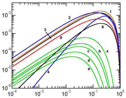
Figure 3. Error curves for approximations with exact extremes and no crossing 

1) Bartolomeu-Michon, 2) Cantrell II, 3) Takakazu Seki, 4) Lockwood, 5) Sykora-Rivera, 6) YNOT, a) Lindner-Selmer and Selmer-Michon, b-e) other combined Padé approximations (see text). The blue error curves (1 and 5) correspond to negative deviations with S'(a,b)<=S(a,b); in all the remaining cases the deviations are non-negative.
 

1) Bartolomeu-Michon approximation

This is an approximation with no adjustable parameters, proposed in 2004 by Ricardo Bartolomeu and refined by G.P.Michon:

(E1)   .

Due to the presence of the atan() function, it belongs to category (C). Its worst error is about 1.72%.

2) Cantrell II approximation

Due to David W. Cantrell, this 2004 approximation is embodied by the formula

(E2)   

with w = 74 and p = 0.2410117.

Though we recognize the presence of the mean R(a,b,w) of Eq.(12), the formula does not fit any of the schemes considered so far and therefore belongs to category B. Its worst error is about 1.42%.

Errata Corrige added on March 15, 2007: I have mistyped the value of p in my Matlab test program. With the correct value of p = 0.410117, this approximation has three zero crossings (class C) and a maximum error of less then 4.2 ppm. Further comments on the [correct] approximation and its error function graph appear in the 2007 Advances ... where it is referred-to as Cantrell 2004.

3) Takakazu Seki approximation

Due to Takakazu Seki Kowa (1642-1708), this is the oldest approximation of the type considered in this Chapter.

(E3)   

It belongs to category (A) since it is obtained starting with the generalized quadratic mean, Eqs.(10,15), and setting w = 8/π² in order to match the perimeter of the degenerate ellipse (b=0). The worst error of this approximation is about 1.35%.

4) Lockwood approximation

(E4)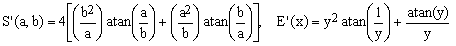   

Like Bartolomeu-Michon, this 1932 approximation also uses tha atan() function and thus belongs to category (C).
Its worst error is about 0.899%.

5) Sykora-Rivera approximation

The following approximation was derived by Sykora in 2005 on the basis of simple symmetry and dimensional considerations:

(E5)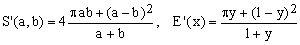   

The name we use here reflects the fact that it matches the first term of an almost contemporary approximation due to D.F.Rivera (see below). Since it is difficult to express this formula in terms of any of the means considered so far, it belongs to category (B). Given its algebraic simplicity, it is very efficient but its maximum error is rather large (about 0.631%).

Note added on February 20, 2006:
This approximation will be henceforth called Cantrell's Particularly Fruitful. See the Comments in the 2006 Addendum for more details.

6) YNOT approximation

This is a very well known approximation due to Roger Maertens (2000) and in a more general form, Necat Tasdelen (1959):

(E6)   

It belongs to category (A) since it is based on the Hölder mean (Eq.11) with its parameter s adjusted so as to exactly match the case y = 0 as well as y = 1. The worst error of the YNOT formula is about 0.362%, twice less than the previous one. Its drawback is the necessity to evaluate three real powers which makes it very inefficient. Despite its great popularity, the YNOT formula should be considered obsolete, especially considering the existence of many approximations which are both more efficient and more precise.

It is interesting that Hölder mean does not lead to separate solutions for minimum overall error and for the exact solution of the limit cases of y = 0 and y=1; in this case, the two optimization criteria both lead to the YNOT formula. This differs markedly from the case of quadratic mean where the two solutions (the optimized quadratic and the Takakazu Seki approximations) are distinct.

a-e) Combined Padé approximations

In the Chapter on Keplerian approximations, we have seen that Padé approximants in terms of the parameter h (Eq.8) offer, all considered, the best compromise between efficiency and precision. Their drawback is that they do not match exactly the extreme case y = 0, a property desirable in many practical applications.

We will now propose a simple and very general method to remove this drawback and show that methods based on Padé approximants turn up once again to be among the most efficient ones.

Consider that one has two different approximations a(y), b(y) for the same function f(y). Their linear combination c(p,y) = p.a(y)+(1-p).b(y) is then again an approximation of f(y) and it contains an adjustable parameter p. Consequently, approximation c(y) can be optimized by adjusting p according to various optimization criteria (such as minimum overall error or exact value at a given point). Notice that if both a(y) and b(y) are exact at a certain point, so is c(y), regardless of the value of p.

In the case of the Keplerian approximations discussed in Chapter 2, a(y) and b(y) could be any pair of approximate formulae. Since all of them are precise for y = 1, so are their linear combinations. The parameter p can be then set to the precise value needed to make the linear combination precise also for y = 0. Evidently, starting with 15 approximations, this would lead to 105 different combinations to explore. Here we shall concentrate only on combinations of consecutive Padé approximation pairs whose error curves, incidentaly, have no zero crossings.

a) Padé 1/2 (Michon) combined with Padé 1/1 (Selmer)

(Ea)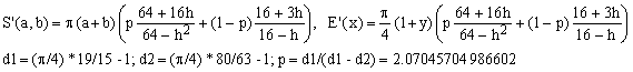   

Here d1 and d2 are the deviations of the two considered approximations for E' from E at y = 0 (corresponding to h = 1 and E = 1). The formula for the parameter p which makes the combination exact at y = 0 is than as shown.

The approximation (Ea) has a maximum error of only 0.060% or 600 ppm which is about 7 times better than YNOT. With respect to YNOT it has the advantage of being computationally much more efficient since it involves only a few basic arithmetic operations.

The amazing thing, however, is that another combination of approximations, namely that of Padé 1/1 (Selmer) with Lindner (K9) is so close to (Ea) that their error curves in Figure 3 cannot be distinguished and its maximum error is nearly identical (615 ppm). The corresponding formulae are

(Ea')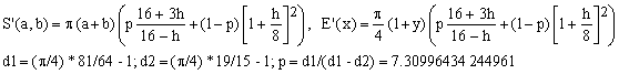   

b) Padé 2/1 (Hudson-Lipka) combined with Padé 1/2 (Michon)

(Eb)   

The worst error of this approximation is about 282 ppm. This is twice better than (Ea) at almost no price in terms of an extra computational effort.

c) Padé 2/2 (Jacobsen-Waadeland) combined with Padé 2/1 (Hudson-Lipka)

(Ec)   

This approximation has the worst error of about 194 ppm - 30% better than (Eb) for a very modest extra computational effort.

d) Padé 3/2 combined with Padé 2/2 (Jacobsen-Waadeland)

(Ed)   

The error of this approximation never exceeds 97 ppm. It is the first of all the approximations discussed so far which breaks the 100 ppm barrier!

e) Padé 3/3 combined with Padé 3/2

(Ee)   

The worst error of this formula is about 54 ppm but its computational complexity is rather high (even though it uses only basic arithmetic operations).

C. Approximations with exact extremes and crossings

We shall now discuss the remaining approximations which are exact for both y = 1 and y = 0 and contain cross points at which S'(a,b) = S(a,b). Since at such points the error is zero, some authors consider the presence of crossings as an advantage and even annotate the y-values at which the deviation vanishes.

On the other hand, crossings usually reveal a somewhat 'unnatural' behaviour of the residual deviation and tend to make further improvements difficult and unlikely. We simply list the known approximations of this type in order of decreasing maximum error.

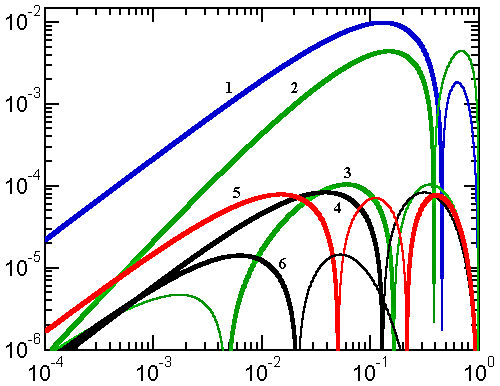
Figure 4. Error curves for approximations with exact extremes and crossings 

1) Bartolomeu, 2) Rivera I, asymmetric, 3) Rivera II, 4) Cantrell I, 5) Sykora, 6) Cantrell-Ramanujan. The thin lobes of each curve correspond to negative deviations with S'(a,b)<=S(a,b) and the thick lobes to non-negative deviations.
 

1) Bartolomeu approximation

(C1)   .

This 2004 formula due to Ricardo Bartolomeu is listed as a curiosity since, with its large maximum error (about 0.98%) and computationally inefficient formula it is no match for many of the approximations we have already seen. What makes it somewhat interesting is its apparent affinity with the sinc function.

2) Rivera I asymmetric approximation

(C2)   .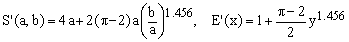

Again, this 2004 formula is reported for the sake of completeness and for curiosity. Its maximum error is 0.45% and it is rather inefficient due to the presence of the power function. Moreover, it is the only one of all the approximations discussed here which requires that b<=a. Such a lack of symmetry under the permutation of a and b is unsatisfactory in most physically meaningful applications.

3) Rivera II approximation

(C3)   .

This is a quite successful 2004 approximation due to David F.Rivera. Its maximum error of only 103 ppm is quite respectable, despite the presence of the square roots.

4) Cantrell approximation

(C4)   .

This 2001 approximation by David W.Cantrell uses, in a bit non-standard way, the Hölder mean with negative exponent. The parameter s can be set to optimize its performance for low-eccentricity ellipses (s = [3*π-8]/[8-2*π]), large-eccentricity ellipses (s = log[2]/log[2/[4-π]]) or to minimize the maximum error (s = 0.825056176207). The error curve shown in Figure 4 corresponds to the latter case and its maximum error value is 83 ppm. The approximation therefore breaks the 100 ppm barrier, but the feat is somewhat diminished by the necessity to evaluate a real power.

5) Sykora approximation

(C5)   .

This 2005 approximation, developed using physical insight, is highly successful considering that it uses a very limited number of simple algebraic operations and its maximum error is jjust 78.5 ppm. Even the combined Padé approximations of comparable precision, (Ed) and (Ee), require a substantially higher number of operations.

6) Cantrell-Ramanujan approximation

(C6)   .

This is so far the most precise approximation, derived in 2004 by D.W.Cantrell from Ramanujan II by adding a correction term which makes it exact at y = 0. The term is proportional to the 12-th power in h which - despite appearances - is quite easy to compute. The efficiency of the formula is somewhat limited by the presence of a square root but its maximum error of only 14.5 ppm is impressive. It also maintains the extremely low error values for low eccentricity ellipses characteristic of Ramanujan II.

Conclusions

The method of comparing various ellipse perimeter approximations based on relative error-curve plots turns out to be very successful. It offers an at-a-glance comparison and makes it possible to classify the multitude of known approximations according to various criteria. This Note attempts one such classification though one can easily imagine many others.

The Author proposes a novel class of rather efficient approximations based on linear combinations of Padé approximants (Ea - Ee) which are precise in both extreme cases of y = b/a = 0 and 1 and feature worst-case errors between 615 ppm and 54 ppm, depending upon the complexity of the formula.

The error curve plots make it easy to compare the various formulae in terms of their maximum error on one side and computational efficiency on the other. In order to keep the length of the article under a reasonable limit the detailed analysis is not reported, but the comparisons between various formulae are quite simple and the results can be easily checked by the reader. It turns out that, after eliminating numerically inefficient approximations containing transcendental functions (with the exception of square-root which implies about 6 divisions and as many additions), the three most efficient approximations are: 
*** Sykora-Rivera (E5) when a maximum error of 0.63% (6300 ppm) is tolerable, or
*** Sykora (C5) when a 79 ppm maximum error is tolerable, or
*** Cantrell-Ramanujan (C6) when a 15 ppm maximum error is acceptable.

The last statement is to be intended in the following way. Suppose that we are looking for the most efficient approximation with maximum error of 500 ppm. Consulting the graphs, one finds that the approximations which satisfy the requirement are: K12, Ke, Kf, Eb, Ec, Ed, Ee, C3, C4, C5 and C6. A simple inspection then reveals that, among these, C5 requires the least computational effort. Repeating this kind of reasoning for various maximum error requirements, the formulae which always turn up are E5, C5 and C6, indicating that they constitute a kind of cardinal points.

Those who wish to pursue this topic further should look for an efficient formula using only the four algebraic operations (if possible, avoiding even square-root) with a maximum error below 10 ppm. If would be also nice if such a formula were exact for both the circle (y=1) and the degenerate flat ellipse (y=0).

As a little contribution to this hunt, I include a small MATLAB program which computes the error curves of all approximations reported in this article. You can use it to add your new formula and plot its error curve as well.

Click here to download the free MATLAB program.