1. Introduction

Apparently, one would think that computing the circumference S of an ellipse with semi-axes a and b is an established task and that one can hardly say anything new about the topic. Assuming a≥b, elementary calculation gives

(1)   

is the ellipse eccentricity and

(2)   

is the complete elliptic integral of the second kind, a well known mathematical entity [4,5,6] which can be computed with relative ease using, for example, brute-force rational approximations [4] or the Carlson's algorithms described in [6].

For a physicist or an engineer, formula (1) is somewhat disappointing because of its apparent asymmetry with respect to the parameters a and b, exacerbated by the condition a≥b. It does not reflect in any straightforward way the quite obvious fact that S(a,b)=S(b,a) is invariant with respect to the permutation of the two semi-axes.

Moreover, we know the exact solutions of two border cases, namely S(a,0)=4a, S(0,b)=4b and S(a,a)=2πa. These extremes (degenerate ellipses and a circle) are accounted for by the values E(1)=1 and E(0)=π/2, but one feels that they should be much more evident directly from the form of the formula.

There exists, however, a number of approximate formulae which do not suffer from the above drawbacks (see the G.P.Michon's review article). Some of these, in particular D.W.Cantrell's, D.F.Rivera's, are also quite precise. From the point of view of the present enquiry, however, even such formulse have an additional drawback. Our final goal is a generalization of the formula, exact or approximate, for the surfaces of n-dimensional ellipsoids of which the ellipse perimeter is just the simplest case (n=2). Unfortunately, neither Eq.(1), nor any of the known approximations are easy to generalize for n>2.

Here we present a method for a derivation of approximations to the ellipse circumference based on the exploitation of border cases (one semi-axis null or all semiaxes equal), symmetry under permutations and the dimensional scaling property. In a subsequent article it will be shown how these same properties can be exploited to handle higher-dimensional cases.

2. Base approximation

In order to maintain the symmetry S(a,b)=S(b,a) and make it more explicit, we shall approximate S(a,b) by means of functions of symmetrized polynomials in a and b. The simplest of such polynomials is (a+b) so that, considering the degenerate cases S(a,0)=4a and S(0,b)=4b, the first term in S(a,b) should be 4(a+b). The residue S(a,b)-4(a+b) then vanishes whenever either a or b is zero, a fact which makes it reasonable to write

(3)   S(a,b) = 4(a+b)+abR₀(a,b),

where R₀(a,b) is a symmetric function of a and b. However, a physicist immediately spots the dimensional incongruity in Eq.[3]. Since S(a,b),a, and b all have a physical dimension of length, R(a,b) must have the dimension of the inverse of length. It therefore appears more appropriate to write

(4)   

where the function A(a,b) is symmetric and a-dimensional (i.e., invariant when both its arguments are scaled by a common factor).

The simplest choice for A(a,b) is a constant k. The special case of S(a,a)=2πa can be now used to determine the value of k, which comes out as 4π-16. With this choice, the first approximation function for S(a,b) becomes

(5)   

and has the advantage of being exact in all special cases. This approximation can not be considered truly new since, for example, it coincides with the first term of a more precise approximation due to D.F.Rivera (a reason why we should call it either Rivera-Sykora or Sykora-Rivera).

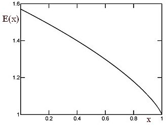
In order to estimate the relative deviation of formula [5] from S(a,b), let us use it to approximate E(x). Considering that

(6)   

Eqs.(1) and (5) lead to the following approximation E₀(x) for E(x):

(7)   

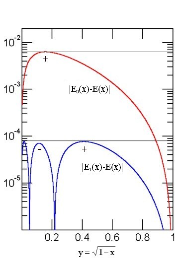
The plot of the relative deviation of the last formula E(x) is shown in the Figure on the right (the red line). Note that the deviations are plotted agains the quantity y of Eq.(7) which allows to show in a visually better way the details of the curves for eccentricities close to 1 (nearly degenerate ellipses).

The graph indicates that the relative deviation never exceeds 0.63%. Considering the algebraic simplicity of the approximation, this is quite good. The behavior of the relative error resembles closely that of the the optimized quadratic formula and that of the slightly better R.Maerten's YNOT formula (see the link to G.P.Michon's article for more details on the mentioned approximations). Eqs.(5) and (7), however, are much simpler and computationally more efficient.

3. Correction term

Considering the success of approximations (5) and (7), we can try and proceed one step further. Since Eq.(5) gives the exact answer when either a=0 or b=0 and also when a=b, and considering the symmetry S(a,b)=S(b,a), we would expect the next correction term to be proportional to ab(a-b)². This is a polynomial in a and b containing only fourth-order terms which, in order to maintain the correct dimensionality of the result, must be divided by a third-order polynomial symmetrical in a,b and containing only third-order terms. All such polynomials are necessarily of the form

(8)   α(a+b)³+β(a²b+b²a) or α(a+b)[(a+b)²+γab],

with α, β and γ some arbitrary constants. Consequently, the expected form of the next correction term is

(9)   

Numeric adjustment of the constants λ and μ has revealed that smallest maximum relative error is achieved in the immediate vicinity of the values λ = -1/2 and μ = π. Hence the following approximations:

(10)   

(11)   

The relative error of the formulae (10) and (11) is again shown in the above Figure (the blue line).

4. Conclusions

It turns out that the magnitude of the relative error of Egs.(10) and (11) never exceeds 78.5 ppm, a precision which is quite satisfactory for most physical and engineering applications and better than the computationally less efficient Cantrell's formula of 2001 (though not as good as the Cantrell's approximation of 2004). Compared with the base approximation, the error has dropped by a factor of about 80, thus illustrating the validity of the adopted approach.

In a forthcoming Note it will be shown that the approach can be extended to n-dimensional ellipsoids with n>2.